Authors:
(1) Nora Schneider, Computer Science Department, ETH Zurich, Zurich, Switzerland ([email protected]);
(2) Shirin Goshtasbpour, Computer Science Department, ETH Zurich, Zurich, Switzerland and Swiss Data Science Center, Zurich, Switzerland ([email protected]);
(3) Fernando Perez-Cruz, Computer Science Department, ETH Zurich, Zurich, Switzerland and Swiss Data Science Center, Zurich, Switzerland ([email protected]).
Table of Links
2 Background
3.1 Comparison to C-Mixup and 3.2 Preserving nonlinear data structure
4 Experiments and 4.1 Linear synthetic data
4.2 Housing nonlinear regression
4.3 In-distribution Generalization
4.4 Out-of-distribution Robustness
5 Conclusion, Broader Impact, and References
A Additional information for Anchor Data Augmentation
A Additional information for Anchor Data Augmentation
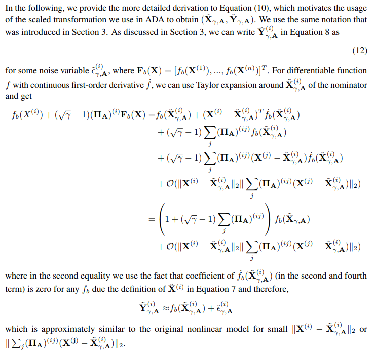
A.1 Derivation of ADA for nonlinear data
A.2 Additional information on hyperparameters of ADA
In this section, we illustrate in a simple 1D example (i.e. cosine data used in Figure 1) how changes in the hyperparameter values modify the data and affect the achieved estimation. Additionally, we show in Appendix B.4 how ADA performance on real-world data is impacted by changes in the hyperparameter values.

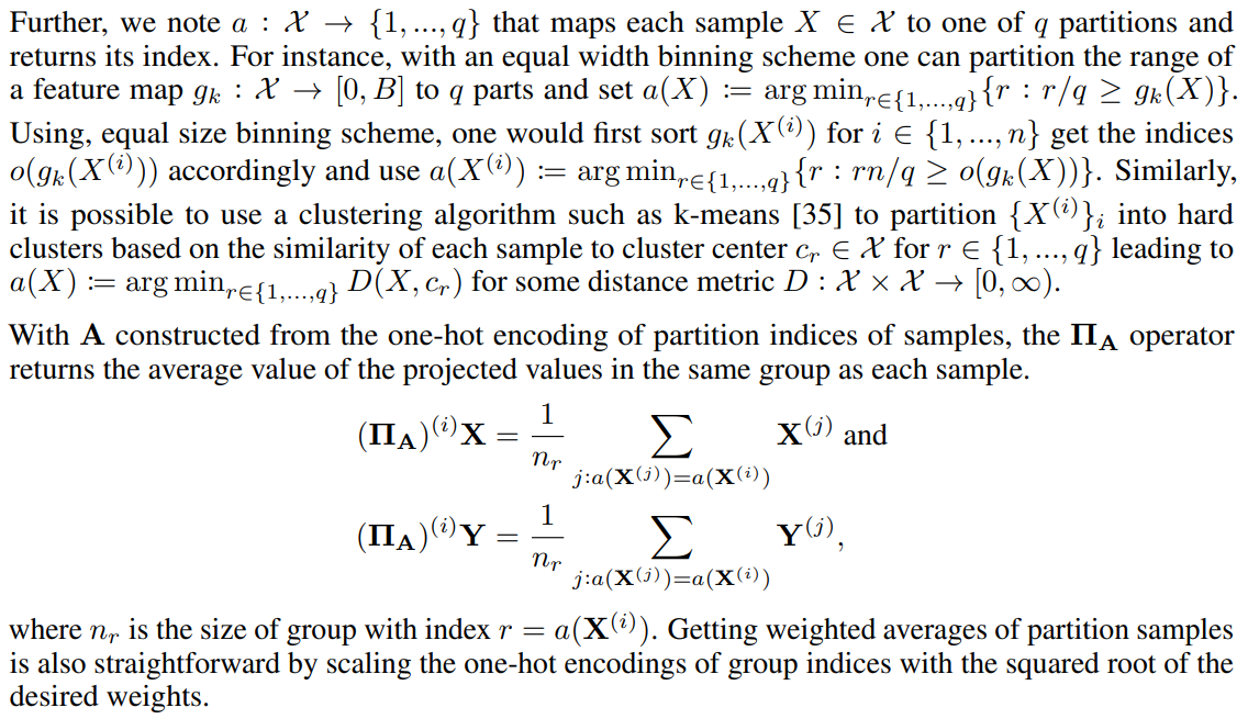
Anchor Matrices and Locality: Anchor variable A is assumed to be the exogenous variable that generates heterogeneity in the target and has an approximately linear relation with (X, y) (see AR loss in Equation 3). It is recommended to choose the variable relying on expert knowledge about the features that the target has a higher dependence on or is possibly misrepresented in the dataset so that we encourage the robustness of the trained model against this type of discrepancy. After deciding the features, one way to construct the anchor matrix A is to partition the dataset according to the similarity of the features, using for example binning or clustering algorithms. Then we can fill the rows of A with a one-hot encoding of the partition index that each sample belongs to.
We use the following nonlinear Cosine data model as a running example to demonstrate more clearly how A is constructed and affects the augmentation procedure.

For illustration purposes, we use in Figures 5, 7 equidistant x values as this reduces noise and emphasizes the effect of ADA parameters more.
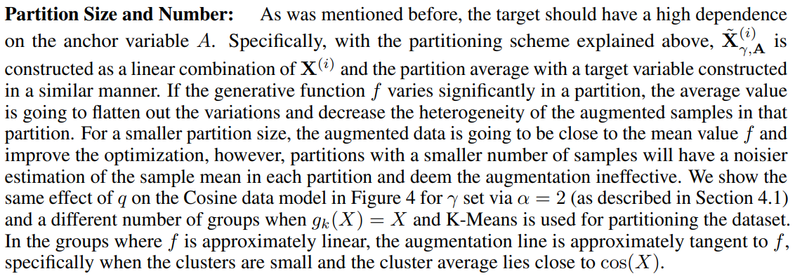
![Figure 4: Model predictions for models fit on the original data and ADA augmented data with varying partition sizes. On a hold-out validation set the base model has MSE = 0.097. The augmented model achieves MSEs of 0.124, 0.069, 0.079, respectively. We use MLPs with architecture [50, 50, 50, 50, 50] and ReLU activation function. The original data has n = 20 points. We use k-means clustering, α = 2, and augmented 10 additional points per given point.](https://cdn.hackernoon.com/images/fWZa4tUiBGemnqQfBGgCPf9594N2-i6d3039.png)

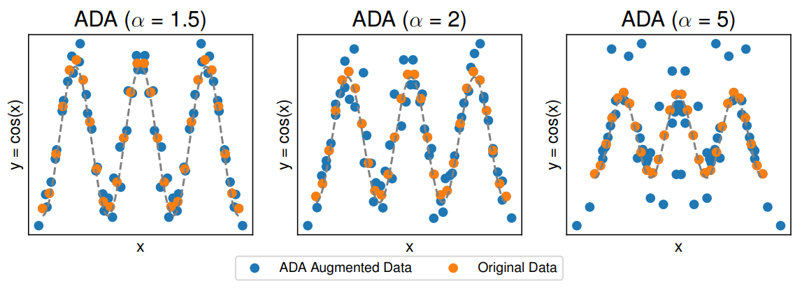
![Figure 6: Model predictions for models fit on the original data and ADA augmented data with different ranges of γ controlled via the parameter α. On a hold-out validation set the base model has MSE = 0.097. The augmented model fits achieve MSEs of 0.083, 0.124, 0.470, respectively. We use MLPs with architecture [50, 50, 50, 50, 50] and ReLU activation function. The original data has n = 20 points. We use k-means clustering into q = 2 groups and augmented 10 additional points per given point.](https://cdn.hackernoon.com/images/fWZa4tUiBGemnqQfBGgCPf9594N2-k8g30qq.png)
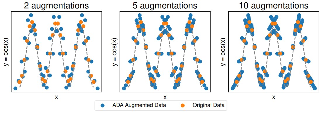
Number of augmentations: For each anchor matrix A and γ we can add n new samples to the dataset. The addition of more augmented samples may not be beneficial as the optimization may overfit the approximations in the augmented data model in Equation 10. In the Cosine data model this is specifically problematic when X is close to multiples of π as depicted in Figure 7. Additionally, we provide a baseline and an augmented model fit in Figure 8 with different number of augmentations.
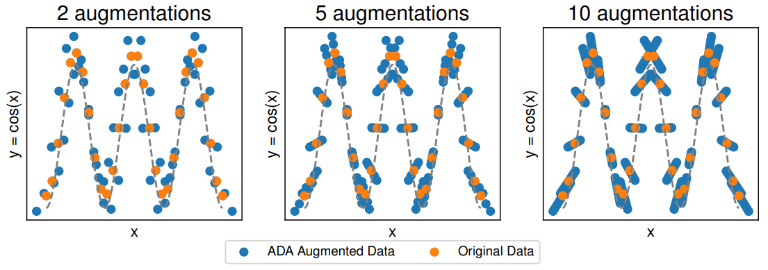
As it is standard practice to use stochastic gradient descent methods for optimizing a regressor, we suggest applying ADA on each minibatch instead of the entire dataset. This avoids choosing a fixed numbers of augmentations. Furthermore, it adds diversity to the "mixing" behavior of ADA, because the samples that are being mixed change in each iteration.
![Figure 8: Model predictions for models fit on the original data and ADA augmented data with a different number of parameter combinations (equal number of augmentations). On a hold-out validation set the base model has MSE = 0.097. The augmented model fits achieve MSEs of 0.470, 0.071, 0.057, respectively. We use MLPs with architecture [50, 50, 50, 50, 50] and ReLU activation function. The original data has n = 20 points. We use k-means clustering into q = 5 groups and α = 2.](https://cdn.hackernoon.com/images/fWZa4tUiBGemnqQfBGgCPf9594N2-w2i30rt.png)
This paper is available on arxiv under CC0 1.0 DEED license.

