Authors:
(1) Nora Schneider, Computer Science Department, ETH Zurich, Zurich, Switzerland ([email protected]);
(2) Shirin Goshtasbpour, Computer Science Department, ETH Zurich, Zurich, Switzerland and Swiss Data Science Center, Zurich, Switzerland ([email protected]);
(3) Fernando Perez-Cruz, Computer Science Department, ETH Zurich, Zurich, Switzerland and Swiss Data Science Center, Zurich, Switzerland ([email protected]).
Table of Links
2 Background
3.1 Comparison to C-Mixup and 3.2 Preserving nonlinear data structure
4 Experiments and 4.1 Linear synthetic data
4.2 Housing nonlinear regression
4.3 In-distribution Generalization
4.4 Out-of-distribution Robustness
5 Conclusion, Broader Impact, and References
A Additional information for Anchor Data Augmentation
B Experiments
B.1 Linear synthetic data
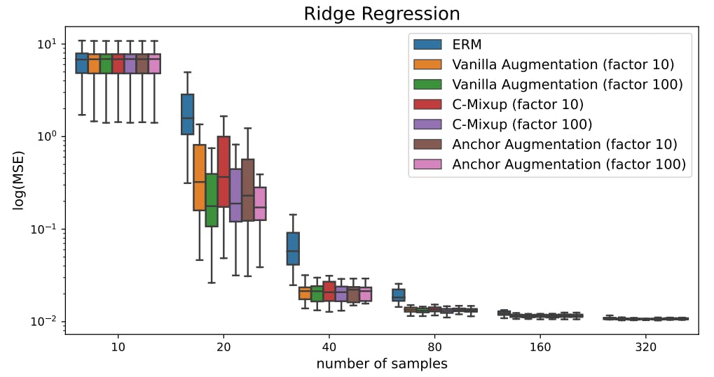
In this section, we present more detailed results of the experiments on synthetic linear data (Section 4.1). First, Figure 9 shows a comparison of using 10 instead of 100 additional augmentations per original sample using Ridge regression model. Performance increases when using 100 instead of 10 augmentations for all methods, as the resulting prediction error is lower.
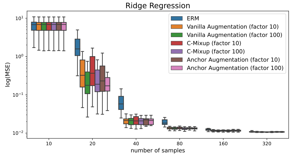
Second, we report experimental results for using a wider interval for γ values in Figure 10. The width is controlled via the parameter α, as described in Section 3. While for ridge regression, the effectiveness of anchor augmentation is not sensitive to the choice of α, the MLP model shows more sensitivity.

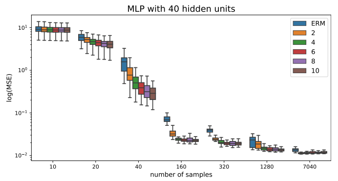
Finally, we report results for using an MLP with 40 hidden units in Figure 11. The results are consistent with the results from the MLP with 10 hidden unity.
B.2 Additional results for real-world regression data
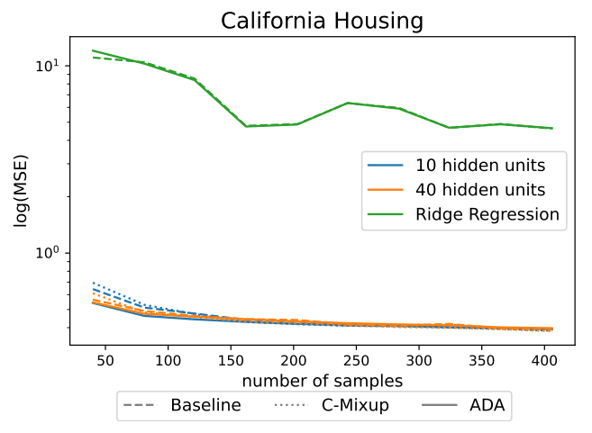
In Figure 12 we provide additional results showing, that the Ridge regression model performs worse on the California housing data. The experimental setting is the same as described in Section 4.2.
B.3 Additional results on real-world data
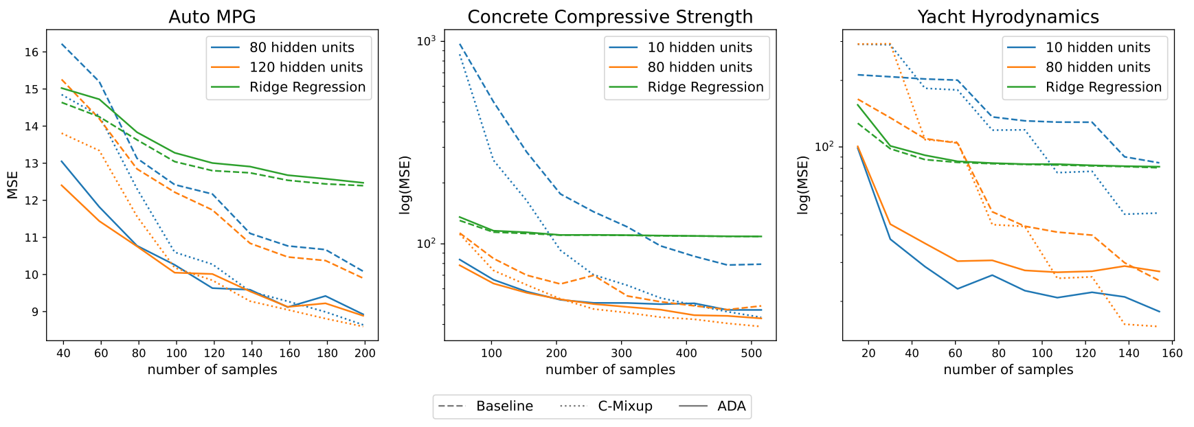
In this section, we provide further experimental results on real-world regression problems. We use the following datasets from the UCI ML repository [12]: Auto MPG (7 predictors), Concrete Compressive Strength(8 predictors), and Yacht Hydrodynamics (6 predictors). The experimental setting follows the one described in Section 4.2, except that we use here to training, validation, and test datasets of relative sizes 50%, 25%, and 25% respectively. We use MLPs with one layer and varying layer width and sigmoid activation. The models are trained using Adam optimization. We generate 9 different dataset splits and report the average prediction error in Figure 13. Similar to the results in Section 4.2, ADA outperforms the baseline and C-Mixup especially when little data is available. The performance gap vanishes when more samples are available demonstrating the effectiveness of ADA in over-parameterized scenarios.
B.4 Details: In-distribution Generalization and Out-of-distribution Robustness
In this section we present details for the experiments described in section 4.3 and Section 4.4. We closely follow the experimental setup of [49].
Data Description
In the following, we provide a more detailed description of the datasets used for in-distribution generalization and out-of-distribution robustness experiments.
Airfoil [12]: is a tabular dataset originating from aerodynamic and acoustic tests of two and three-dimensional airfoil blade sections. Each input has 5 features measuring frequency, angle of attack, chord length, free-stream velocity and suction side displacement thickness. The target variable is the scaled sound pressure level. As in [49], we additionally apply Min-Max normalization on the input featues and split the dataset into train (1003 samples), validation (300 samples) and test (200 samples) data.
NO2: is a tabular dataset originating from a study where air pollution at a road is related to traffic volume and meteorological variables. Each input has 7 features measuring, the logarithm of the number of cars per hour, temperature 2 meter above ground, wind speed, the temperature difference between 25 and 2 meters above ground, wind direction, hour of day and day number from 1st October 1 2001. The target variable is the logarithm of the concentration of NO2 particles, measured at Alnabru in Oslo, Norway. Following [49], we split the dataset into a train (200 samples), validation (200 samples) and test data (100 samples).
Exchange-Rate [27]: is a timeseries measuring the daily exchange rate of eight foreign countries including Australia, British, Canada, Switzerland, China, Japan, New Zealand and Singapore ranging from 1990 to 2016. The slide window size is 168 days, therefore the input has dimension 168 × 8 and the label has dimension 1 × 8. Following [27, 49] the dataset is split into training (4,373 samples), validation (1,518 samples) and test data (1,518 samples) in chronological order.
Electricity [27]: is a timeseries measuring the electricity consumption of 321 clients from 2012 to 2014. Similar to [27, 49] we converted the data to reflect hourly consumption. The slide window size is 168 hours, therefore the input has dimension 168 × 321 and the label has dimension 1 × 321. The dataset is split into training (15,591 samples), validation (5,261 samples) and test data (5,261 samples) in chronological order.
RCF-MNIST [49]: is rotated and colored version of F-MNIST simulating a subpopulation shift. The author rotate the images by a normalized angle g ∈ [0, 1]. In the training data they additionally color 80% of images with RGB values [g; 0; 1 − g] and 20% of images with RGB values [1 − g; 0; g]. In the test data, they reverse the spurious correlations, so 80% of images are colored with RGB values [1 − g; 0; g] and the remaining are colored with [g; 0; 1 − g].
Crime [12]: is a tabular dataset combining socio-economic data from the 1990 US Census, law enforcement data from the 1990 US LEMAS survey, and crime data from the 1995 FBI UCR. Each input has 122 features that are supposed to have a plausible connection to crime, e.g. the median family income or per capita number of police officers. The target variable is the per capita violent crimes, representing the sum of violent crimes in the US including murder, rape, robbery, and assault. Following [49], we normalize all numerical features to the range [0.0, 1.0] by equal-interval binning method and we impute the missing values using the mean value of the respective attribute. The state identifications are used as domain information. In total, there are 46 distinct domains and the data is split into disjoint domains. More precise, the training data has 1, 390samples with 31 domains, the validation data has 231 sampels with 6 domains and the test data has 373 samples with 9 domains.
SkillCraft [12]: is a tabular dataset originating from a study which uses video game from real-time strategy (RTS) games to explore the development of expertise. Each input has 17 features measuring player-related parameters, e.g. the age of the player and Hotkey usage variables. Following [49], we use the action latency in the game as a target variable. Missing values are imputed using the mean value of the respective attribute. "League Index", which corresponds to different levels of competitors, is used as domain information. In total there are 8 distinct domains and the data is split into disjoint domains. More precise, the training data has 1, 878 samples with 4 domains, the validation data has 806 samples with 1 domain and the test data has 711 samples with 3 distinct domains.
DTI [17]: is a tabular dataset where the target is the binding activity score between a drug molecule and the corresponding target protein. The input consists of 32, 300 features which represent a onehot encoding of drug and target protein information. Following [49], we use "Year" as domain information with 8 distinct domains. There are 38, 400 training, 13, 440 validation and 11, 008 test samples.
Methods and Hyperparameters
For ERM, Mixup, ManiMixup and C-Mixup, we apply the same hyperparameters as reported in the original C-Mixup paper [49]. According to the authors they are already finetuned via a cross validation grid search. The details can be found in the corresponding original paper. We rerun their experiments with the provided repository (https://github.com/huaxiuyao/C-Mixup) over three different seeds ∈ {0, 1, 2}. Furthermore, we finetune ADA and training hyperparameters using a grid search. The detailed hyperparameters for in-distribution generalization and out-of-distribution robustness are reported in Table 3. We apply ADA using the same seeds.

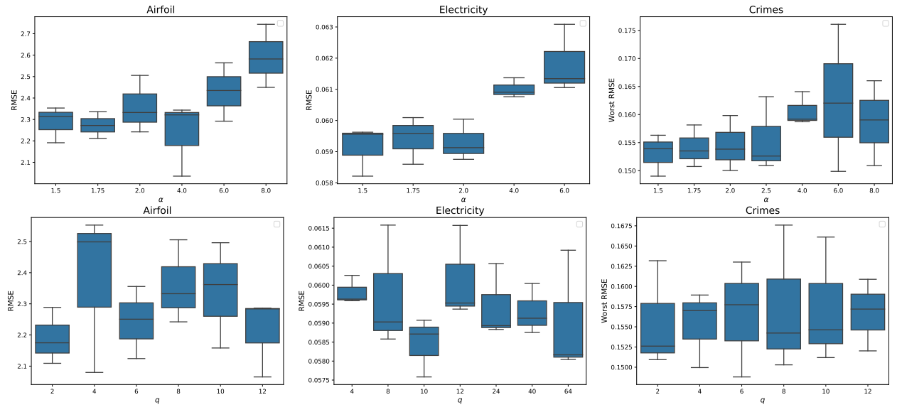
Furthermore, we provide the performance of ADA for different parameter parameter values to get a better understanding of their impact. We vary values for q, the number of clusters used in k-means clustering, and α, the parameter that controls the range of γ-values on selected in-distribution and out-of-distribution datasets. Results are reported in Figure 14.
Detailed Results
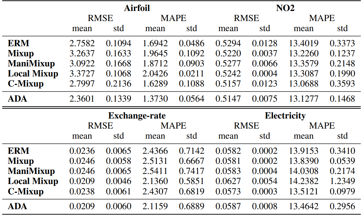
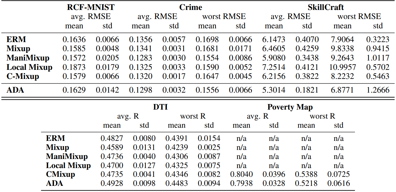
We report the results for in-distribution generalization experiments in Table 4 and for out-of-distribution generalization experiments in Table 5. Following [49], we further evaluated the performance of ADA and C-Mixup on the Poverty dataset [23], which contains satellite images from African countries and the corresponding village-level real-valued asset wealth index. Again we closely followed the experimental setup, so for details we refer to [49]. However, due to computational complexity, ADA hyperparameters are not tuned on this dataset. We use the same learning parameters as reported in [49] and q = 24 and α = 2.
This paper is available on arxiv under CC0 1.0 DEED license.

